# A tibble: 3 × 6
     id `count/num`   W.t Case  `time--d` `%percent`
  <int> <chr>       <int> <chr>     <int>      <int>
1     1 china           3 w             5         25
2     2 us              4 f             6         34
3 3 india 5 q 8 78附录 G — 其它有趣的包
G.1 janitor包
整理、清洗数据的好上手的包。
G.1.1 整理列名
fake_raw %>%
  janitor::clean_names()
# A tibble: 3 × 6
id count_num w_t case time_d percent_percent
<int> <chr> <int> <chr> <int> <int>
1 1 china 3 w 5 25
2 2 us 4 f 6 34
3 3 india 5 q 8 78
G.1.2 与count()函数对比
  cyl  n percent
1   8 14    43.8
2   4 11    34.4
3   6  7    21.9
G.2 粘贴小表格datapasta包
- 安装install.packages(“datapasta”)
- 鼠标选中并复制网页中的表格
- 在 Rstudio 中的Addins找到datapasta,并点击paste as tribble
G.3 搞定模型公式
library(equatiomatic)
mod1 <- lm(mpg ~ cyl + disp, mtcars)
extract_eq(mod1)
\[ \operatorname{mpg} = \alpha + \beta_{1}(\operatorname{cyl}) + \beta_{2}(\operatorname{disp}) + \epsilon \]
extract_eq(mod1, use_coefs = TRUE)\[ \operatorname{\widehat{mpg}} = 34.66 - 1.59(\operatorname{cyl}) - 0.02(\operatorname{disp}) \]
G.4 自动搞定报告
G.4.1 生成报告
# A tibble: 3 × 5
  term              estimate std.error statistic   p.value
  <chr>                <dbl>     <dbl>     <dbl>     <dbl>
1 (Intercept)           5.01    0.0728     68.8  1.13e-113
2 Speciesversicolor     0.93    0.103       9.03 8.77e- 16
3 Speciesvirginica 1.58 0.103 15.4 2.21e- 32report(model)We fitted a linear model (estimated using OLS) to predict Sepal.Length with
Species (formula: Sepal.Length ~ Species). The model explains a statistically
significant and substantial proportion of variance (R2 = 0.62, F(2, 147) =
119.26, p < .001, adj. R2 = 0.61). The model's intercept, corresponding to
Species = setosa, is at 5.01 (95% CI [4.86, 5.15], t(147) = 68.76, p < .001).
Within this model:
- The effect of Species [versicolor] is statistically significant and positive
(beta = 0.93, 95% CI [0.73, 1.13], t(147) = 9.03, p < .001; Std. beta = 1.12,
95% CI [0.88, 1.37])
- The effect of Species [virginica] is statistically significant and positive
(beta = 1.58, 95% CI [1.38, 1.79], t(147) = 15.37, p < .001; Std. beta = 1.91,
95% CI [1.66, 2.16])
Standardized parameters were obtained by fitting the model on a standardized
version of the dataset. 95% Confidence Intervals (CIs) and p-values were
computed using a Wald t-distribution approximation.G.4.2 自动模型评估
library(performance)
model <- lm(mpg ~ wt * cyl + gear, data = mtcars)
performance::check_model(model)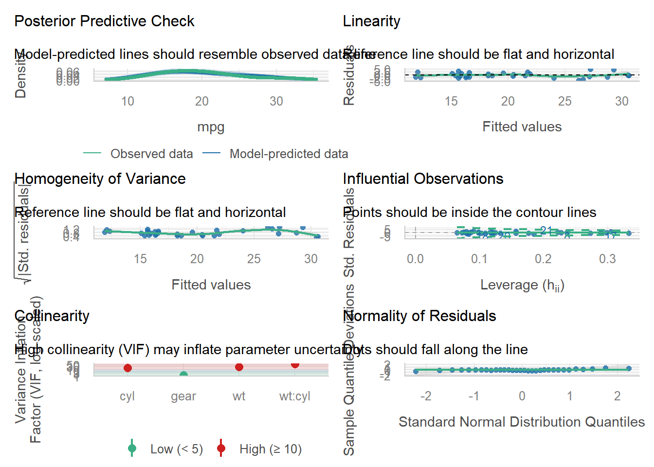
G.4.3 统计表格
library(gtsummary)
gtsummary::trial %>%
  dplyr::select(trt, age, grade, response) %>%
  gtsummary::tbl_summary(
    by = trt,
    missing = "no"
  ) %>%
  gtsummary::add_p() %>%
  gtsummary::add_overall() %>%
  gtsummary::add_n() %>%
gtsummary::bold_labels()| Characteristic | N |
Overall N = 2001 |
Drug A N = 981 |
Drug B N = 1021 |
p-value2 |
|---|---|---|---|---|---|
| Age | 189 | 47 (38, 57) | 46 (37, 60) | 48 (39, 56) | 0.7 |
| Grade | 200 | 0.9 | |||
| I | 68 (34%) | 35 (36%) | 33 (32%) | ||
| II | 68 (34%) | 32 (33%) | 36 (35%) | ||
| III | 64 (32%) | 31 (32%) | 33 (32%) | ||
| Tumor Response | 193 | 61 (32%) | 28 (29%) | 33 (34%) | 0.5 |
| 1 Median (Q1, Q3); n (%) | |||||
| 2 Wilcoxon rank sum test; Pearson’s Chi-squared test | |||||
trial %>%
  select(trt, age, grade) %>%
  tbl_summary(
    by = trt,
    missing = "no",
    statistic = all_continuous() ~ "{median} ({p25}, {p75})"
  ) %>%
  modify_header(
    all_stat_cols() ~ "**{level}**<br>N = {n} ({style_percent(p)}%)"
  ) %>%
  add_n() %>%
  bold_labels() %>%
modify_spanning_header(all_stat_cols() ~ "**Chemotherapy Treatment**")| Characteristic | N |
Chemotherapy Treatment
|
|
|---|---|---|---|
|
Drug A N = 98 (49%)1 |
Drug B N = 102 (51%)1 |
||
| Age | 189 | 46 (37, 60) | 48 (39, 56) |
| Grade | 200 | ||
| I | 35 (36%) | 33 (32%) | |
| II | 32 (33%) | 36 (35%) | |
| III | 31 (32%) | 33 (32%) | |
| 1 Median (Q1, Q3); n (%) | |||