21 迭代

library(tidyverse)

R循环更建议使用purrr的泛函式循环迭代。数学上，函数的函数成为泛函；编程语言中，泛函表示一个函数作用在另一个函数上，通俗的讲就是一个函数作为另一个函数的参数传入。

21.1 across()函数

21.1.1 across()的基本形式

dplyr::across()函数用于在dplyr的mutate()、summarise()等函数中，对数据框的多列同时应用某个函数。

across()有三个主要的参数，across(.cols, .fns, .nams)：

.cols选取列，和select()的用法非常一致:可以使用 starts_with() 和 ends_with() 等函数按列名选择列。此外还有两个在 across() 中非常实用的选择器：everything() 和 where()。
- everything()会选择未被分组的全部列。如果某列已经用来分组(group_by()包裹起来的)，就不会成为across()的对象。
- where()按照列的数据类型选择列。
.fns，指定对所选列需要执行的函数。可以使默认函数，purrr风格匿名函数，以及一个函数列表（这个列表中也可以同时存在默认函数和匿名函数）。
.names，指定所计算新列的列名，主要针对.fns为一个函数列表时使用。如果.fns是多个函数，就在数据列的列名后面跟上函数名，比如"{.col}_{.fn}"；当然，我们也可以简单调整列名和函数之间的顺序或者增加一个标识的字符串，比如弄成"{.fn}_{.col}"，"{.col}_{.fn}_aa"。
- .names 参数在配合 mutate() 使用时尤为重要。默认情况下，across() 的输出会覆盖原列。如要保留原列并创建新列，可以自定义列名。

# 生成包含NA的数据集
set.seed(1014)
rnorm_na <- function(n, n_na, mean = 0, sd = 1) {
  sample(c(rnorm(n - n_na, mean = mean, sd = sd), rep(NA, n_na)))
}
df_miss <- tibble(
  a = rnorm_na(5, 1), # 生成5个数，其中1个NA
  b = rnorm_na(5, 1),
  c = rnorm_na(5, 2),
  d = rnorm(5)
)

# 计算中位数并统计缺失值个数
df_miss |>
  summarise(
    across(
      a:d,
      list(
        median = \(x) median(x, na.rm = T),
        n_miss = \(x) sum(is.na(x))
      ),
      .names = "{.fn}_{.col}"
    ),
    n = n()
  )

# A tibble: 1 × 9
  median_a n_miss_a median_b n_miss_b median_c n_miss_c median_d n_miss_d     n
     <dbl>    <int>    <dbl>    <int>    <dbl>    <int>    <dbl>    <int> <int>
1   -0.703        1   -0.265        1   -0.522        2    0.413        0     5

21.1.2 across()用于自定义函数

across()支持在函数编程中处理多个列。

expand_dates <- function(df) {
  df |>
    mutate(
      across(
        where(is.Date),
        list(year = year, month = month, dat = mday)
      )
    )
}

df_date <- tibble(
  name = c("Amy", "Bob"),
  date = ymd(c("2009-08-03", "2010-01-16"))
)

df_date |>
  expand_dates()

# A tibble: 2 × 5
  name  date       date_year date_month date_dat
  <chr> <date>         <dbl>      <dbl>    <int>
1 Amy   2009-08-03      2009          8        3
2 Bob   2010-01-16      2010          1       16

across()的第一个参数.col使用了整洁选择，这个特性使得在一个参数中提供多列变得容易。以下函数默认计算数值列的均值。但通过提供第二个参数，我们可以选择只汇总选定的列。

summarise_means <- function(df, summary_vars = where(is.numeric)) {
  df |>
    summarise(
      across({{ summary_vars }}, \(x) mean(x, na.rm = T)),
      n = n(),
      .groups = "drop"
    )
}

# 计算所有数值列均值
diamonds |>
  group_by(cut) |>
  summarise_means()

# A tibble: 5 × 9
  cut       carat depth table price     x     y     z     n
  <ord>     <dbl> <dbl> <dbl> <dbl> <dbl> <dbl> <dbl> <int>
1 Fair      1.05   64.0  59.1 4359.  6.25  6.18  3.98  1610
2 Good      0.849  62.4  58.7 3929.  5.84  5.85  3.64  4906
3 Very Good 0.806  61.8  58.0 3982.  5.74  5.77  3.56 12082
4 Premium   0.892  61.3  58.7 4584.  5.97  5.94  3.65 13791
5 Ideal     0.703  61.7  56.0 3458.  5.51  5.52  3.40 21551

# 计算carat、x、y、z列的均值
diamonds |>
  group_by(cut) |>
  summarise_means(c(carat, x:z))

# A tibble: 5 × 6
  cut       carat     x     y     z     n
  <ord>     <dbl> <dbl> <dbl> <dbl> <int>
1 Fair      1.05   6.25  6.18  3.98  1610
2 Good      0.849  5.84  5.85  3.64  4906
3 Very Good 0.806  5.74  5.77  3.56 12082
4 Premium   0.892  5.97  5.94  3.65 13791
5 Ideal     0.703  5.51  5.52  3.40 21551

21.2 批量筛选行

dplyr 提供了 if_any() 和 if_all() 两个变体函数用于与filter()连用筛选行。

df_miss |>
  filter(if_any(a:d, is.na))

# A tibble: 2 × 4
      a      b     c     d
  <dbl>  <dbl> <dbl> <dbl>
1 -2.44 -0.244    NA 0.724
2 NA    NA        NA 2.35

df_miss |>
  filter(if_all(a:d, is.na))

# A tibble: 0 × 4
# ℹ 4 variables: a <dbl>, b <dbl>, c <dbl>, d <dbl>

21.3 读取多个文件

本节使用purrr::map()函数批量读取多个文件，并将它们合并为一个数据框。

注记

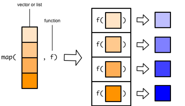
循环迭代，本质上就是将一个函数依次应用（映射）到序列的每一个元素上，表示出来即purrr::map_*(x, f)：序列（用x表示）：由一系列可以根据位置索引的元素构成。通俗的讲，向量、列表、数据框都是序列。
purrr泛函式编程解决循环迭代问题的逻辑：
- 针对序列每个单独的元素的处理，定义为函数
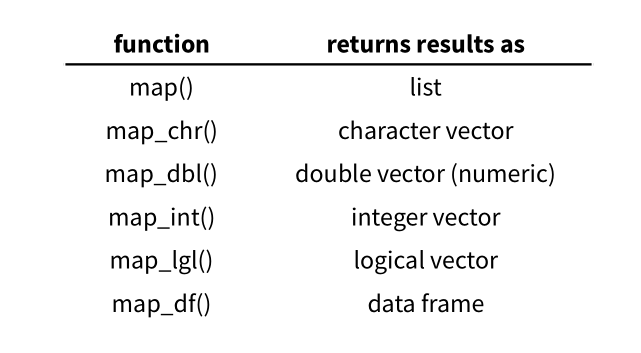
- 在使用map_*()系列函数将定义的函数映射到序列每一个元素上
- 将得到的结果打包一起返回，通过map()函数的后缀控制

其它purrr函数：
- walk_*()系列：只循环迭代，不返回结果。例如用在批量保存数据/图形到文件
- imap_*()系列：元素与索引一起迭代
- modify_*()系列：原地依次修改序列对象
- reduce()/accumlate()：可以先对序列的前两个元素应用函数，在对结果与第三个元素应用函数，在对结果与第四个元素应用函数，……，前者只返回最终结果，后者会返回中间的所有结果

21.3.1 列出目录中的所有文件

list.files() 可以列出目录中的文件，常用参数：

path：目录路径。
pattern：用正则表达式筛选文件名（如 [.]xlsx$ 匹配 .xlsx 文件）。
full.names：是否包含完整路径（建议设为 TRUE）。

path <- list.files("D:/Document/0.Study R/0.R4DS/data/gapminder/", pattern = "[.]xlsx$", full.names = TRUE)
path

 [1] "D:/Document/0.Study R/0.R4DS/data/gapminder/1952.xlsx"
 [2] "D:/Document/0.Study R/0.R4DS/data/gapminder/1957.xlsx"
 [3] "D:/Document/0.Study R/0.R4DS/data/gapminder/1962.xlsx"
 [4] "D:/Document/0.Study R/0.R4DS/data/gapminder/1967.xlsx"
 [5] "D:/Document/0.Study R/0.R4DS/data/gapminder/1972.xlsx"
 [6] "D:/Document/0.Study R/0.R4DS/data/gapminder/1977.xlsx"
 [7] "D:/Document/0.Study R/0.R4DS/data/gapminder/1982.xlsx"
 [8] "D:/Document/0.Study R/0.R4DS/data/gapminder/1987.xlsx"
 [9] "D:/Document/0.Study R/0.R4DS/data/gapminder/1992.xlsx"
[10] "D:/Document/0.Study R/0.R4DS/data/gapminder/1997.xlsx"
[11] "D:/Document/0.Study R/0.R4DS/data/gapminder/2002.xlsx"
[12] "D:/Document/0.Study R/0.R4DS/data/gapminder/2007.xlsx"

21.3.2 读取多个Excel文件并合并

files <- map(path, readxl::read_excel) |>
  list_rbind()
files

# A tibble: 1,704 × 5
   country     continent lifeExp      pop gdpPercap
   <chr>       <chr>       <dbl>    <dbl>     <dbl>
 1 Afghanistan Asia         28.8  8425333      779.
 2 Albania     Europe       55.2  1282697     1601.
 3 Algeria     Africa       43.1  9279525     2449.
 4 Angola      Africa       30.0  4232095     3521.
 5 Argentina   Americas     62.5 17876956     5911.
 6 Australia   Oceania      69.1  8691212    10040.
 7 Austria     Europe       66.8  6927772     6137.
 8 Bahrain     Asia         50.9   120447     9867.
 9 Bangladesh  Asia         37.5 46886859      684.
10 Belgium     Europe       68    8730405     8343.
# ℹ 1,694 more rows

21.3.3 路径中的数据

有时文件名本身包含的有用信息并未在单个文件中记录。为了将该信息添加到最终的数据框中，需要执行两步操作：

用 set_names() 函数为路径向量命名。set_names() 可以接受一个函数作为参数。
接着使用 list_rbind() 的 names_to 参数将这些名称保存为新列，再用 readr::parse_number() 从字符串中提取数值部分。

path |>
  set_names(basename) |> # 从完整路径中提取文件名
  map(readxl::read_excel) |>
  list_rbind(names_to = "year") |>
  mutate(year = parse_number(year))

# A tibble: 1,704 × 6
    year country     continent lifeExp      pop gdpPercap
   <dbl> <chr>       <chr>       <dbl>    <dbl>     <dbl>
 1  1952 Afghanistan Asia         28.8  8425333      779.
 2  1952 Albania     Europe       55.2  1282697     1601.
 3  1952 Algeria     Africa       43.1  9279525     2449.
 4  1952 Angola      Africa       30.0  4232095     3521.
 5  1952 Argentina   Americas     62.5 17876956     5911.
 6  1952 Australia   Oceania      69.1  8691212    10040.
 7  1952 Austria     Europe       66.8  6927772     6137.
 8  1952 Bahrain     Asia         50.9   120447     9867.
 9  1952 Bangladesh  Asia         37.5 46886859      684.
10  1952 Belgium     Europe       68    8730405     8343.
# ℹ 1,694 more rows

在更复杂情形中，目录名中可能含有多个信息片段。此时使用 set_names()（不加参数）保留完整路径，并结合 tidyr::separate_wider_delim()等函数将其拆分为新列。

path |>
  set_names() |>
  map(readxl::read_excel) |>
  list_rbind(names_to = "year") |>
  separate_wider_delim(
    year,
    delim = "/",
    names = c(NA, NA, NA, NA, NA, "dir", "file")
  ) |>
  separate_wider_delim(
    file,
    delim = ".",
    names = c("file", "ext")
  )

# A tibble: 1,704 × 8
   dir       file  ext   country     continent lifeExp      pop gdpPercap
   <chr>     <chr> <chr> <chr>       <chr>       <dbl>    <dbl>     <dbl>
 1 gapminder 1952  xlsx  Afghanistan Asia         28.8  8425333      779.
 2 gapminder 1952  xlsx  Albania     Europe       55.2  1282697     1601.
 3 gapminder 1952  xlsx  Algeria     Africa       43.1  9279525     2449.
 4 gapminder 1952  xlsx  Angola      Africa       30.0  4232095     3521.
 5 gapminder 1952  xlsx  Argentina   Americas     62.5 17876956     5911.
 6 gapminder 1952  xlsx  Australia   Oceania      69.1  8691212    10040.
 7 gapminder 1952  xlsx  Austria     Europe       66.8  6927772     6137.
 8 gapminder 1952  xlsx  Bahrain     Asia         50.9   120447     9867.
 9 gapminder 1952  xlsx  Bangladesh  Asia         37.5 46886859      684.
10 gapminder 1952  xlsx  Belgium     Europe       68    8730405     8343.
# ℹ 1,694 more rows

21.3.4 多次简单迭代

上述示例碰巧读取的是整洁的数据集，大多数情况下需要额外的清理工作。有两种清理方法：用一个复杂的函数进行一次迭代，或是用多个简单函数进行多轮迭代。实践中，往往分步执行更易于调试和维护，也可以让代码的质量更高。

例如，要读取多个文件，过滤缺失值，转换数据格式（pivot），然后合并成一个数据集。更建议的做法是将每一步分别应用到所有文件上，然后再合并结果，更易形成整体视角，并在最终得到更高质量的结果。

paths |>
  map(read_csv) |>
  map(\(df) df |> filter(!is.na(value))) |>
  map(\(df) df |> mutate(id = tolower(id))) |>
  map(\(df) df |> pivot_wider(names_from = id, values_from = value)) |>
  list_rbind()

21.3.5 异构数据

有时数据框之间结构差异太大，导致无法直接用 map() 及 list_rbind()，要么报错，要么合并出一个没法用的结果。

遇到异构数据：

第一步依然是先把所有文件读入
接下来，需要将这些数据框的结构单独提取，以便进一步分析。
最后，针对每种结构分别处理，然后再合并。

21.3.6 错误处理

有时数据结构太复杂，甚至无法一次性读取所有文件。此时 map() 可能会暴露出其弊端：要么所有文件都读取成功，要么因为某个错误一个都不读。

为解决此问题，purrr提供了一个函数操作器：possibly()，可以修改函数的默认行为，使其在出错时返回一个指定的值，而不是抛出错误。

files <- path |>
  map(possibly(\(path) readxl::read_excel(path), NULL))

data <- files |> list_rbind()

failed <- map_vec(files, is.null)
path[failed]

character(0)

以上代码中：

read_excel() 会读取每个文件，若失败则返回 NULL，不会中断整个流程。
list_rbind() 会自动忽略 NULL。
map_vec(files, is.null)找出失败文件的路径，然后对这些失败文件逐一排查，进一步诊断失败原因并做出相应处理。

21.4 几个例子

21.4.1 例1 对数据框逐列迭代

数据框是序列，第1个元素是第1列df[[1]]，第2个元素是第二列df[[2]]：

library(tidyverse)
# 提取
df <- iris[, 1:4]
df

    Sepal.Length Sepal.Width Petal.Length Petal.Width
1            5.1         3.5          1.4         0.2
2            4.9         3.0          1.4         0.2
3            4.7         3.2          1.3         0.2
4            4.6         3.1          1.5         0.2
5            5.0         3.6          1.4         0.2
6            5.4         3.9          1.7         0.4
7            4.6         3.4          1.4         0.3
8            5.0         3.4          1.5         0.2
9            4.4         2.9          1.4         0.2
10           4.9         3.1          1.5         0.1
11           5.4         3.7          1.5         0.2
12           4.8         3.4          1.6         0.2
13           4.8         3.0          1.4         0.1
14           4.3         3.0          1.1         0.1
15           5.8         4.0          1.2         0.2
16           5.7         4.4          1.5         0.4
17           5.4         3.9          1.3         0.4
18           5.1         3.5          1.4         0.3
19           5.7         3.8          1.7         0.3
20           5.1         3.8          1.5         0.3
21           5.4         3.4          1.7         0.2
22           5.1         3.7          1.5         0.4
23           4.6         3.6          1.0         0.2
24           5.1         3.3          1.7         0.5
25           4.8         3.4          1.9         0.2
26           5.0         3.0          1.6         0.2
27           5.0         3.4          1.6         0.4
28           5.2         3.5          1.5         0.2
29           5.2         3.4          1.4         0.2
30           4.7         3.2          1.6         0.2
31           4.8         3.1          1.6         0.2
32           5.4         3.4          1.5         0.4
33           5.2         4.1          1.5         0.1
34           5.5         4.2          1.4         0.2
35           4.9         3.1          1.5         0.2
36           5.0         3.2          1.2         0.2
37           5.5         3.5          1.3         0.2
38           4.9         3.6          1.4         0.1
39           4.4         3.0          1.3         0.2
40           5.1         3.4          1.5         0.2
41           5.0         3.5          1.3         0.3
42           4.5         2.3          1.3         0.3
43           4.4         3.2          1.3         0.2
44           5.0         3.5          1.6         0.6
45           5.1         3.8          1.9         0.4
46           4.8         3.0          1.4         0.3
47           5.1         3.8          1.6         0.2
48           4.6         3.2          1.4         0.2
49           5.3         3.7          1.5         0.2
50           5.0         3.3          1.4         0.2
51           7.0         3.2          4.7         1.4
52           6.4         3.2          4.5         1.5
53           6.9         3.1          4.9         1.5
54           5.5         2.3          4.0         1.3
55           6.5         2.8          4.6         1.5
56           5.7         2.8          4.5         1.3
57           6.3         3.3          4.7         1.6
58           4.9         2.4          3.3         1.0
59           6.6         2.9          4.6         1.3
60           5.2         2.7          3.9         1.4
61           5.0         2.0          3.5         1.0
62           5.9         3.0          4.2         1.5
63           6.0         2.2          4.0         1.0
64           6.1         2.9          4.7         1.4
65           5.6         2.9          3.6         1.3
66           6.7         3.1          4.4         1.4
67           5.6         3.0          4.5         1.5
68           5.8         2.7          4.1         1.0
69           6.2         2.2          4.5         1.5
70           5.6         2.5          3.9         1.1
71           5.9         3.2          4.8         1.8
72           6.1         2.8          4.0         1.3
73           6.3         2.5          4.9         1.5
74           6.1         2.8          4.7         1.2
75           6.4         2.9          4.3         1.3
76           6.6         3.0          4.4         1.4
77           6.8         2.8          4.8         1.4
78           6.7         3.0          5.0         1.7
79           6.0         2.9          4.5         1.5
80           5.7         2.6          3.5         1.0
81           5.5         2.4          3.8         1.1
82           5.5         2.4          3.7         1.0
83           5.8         2.7          3.9         1.2
84           6.0         2.7          5.1         1.6
85           5.4         3.0          4.5         1.5
86           6.0         3.4          4.5         1.6
87           6.7         3.1          4.7         1.5
88           6.3         2.3          4.4         1.3
89           5.6         3.0          4.1         1.3
90           5.5         2.5          4.0         1.3
91           5.5         2.6          4.4         1.2
92           6.1         3.0          4.6         1.4
93           5.8         2.6          4.0         1.2
94           5.0         2.3          3.3         1.0
95           5.6         2.7          4.2         1.3
96           5.7         3.0          4.2         1.2
97           5.7         2.9          4.2         1.3
98           6.2         2.9          4.3         1.3
99           5.1         2.5          3.0         1.1
100          5.7         2.8          4.1         1.3
101          6.3         3.3          6.0         2.5
102          5.8         2.7          5.1         1.9
103          7.1         3.0          5.9         2.1
104          6.3         2.9          5.6         1.8
105          6.5         3.0          5.8         2.2
106          7.6         3.0          6.6         2.1
107          4.9         2.5          4.5         1.7
108          7.3         2.9          6.3         1.8
109          6.7         2.5          5.8         1.8
110          7.2         3.6          6.1         2.5
111          6.5         3.2          5.1         2.0
112          6.4         2.7          5.3         1.9
113          6.8         3.0          5.5         2.1
114          5.7         2.5          5.0         2.0
115          5.8         2.8          5.1         2.4
116          6.4         3.2          5.3         2.3
117          6.5         3.0          5.5         1.8
118          7.7         3.8          6.7         2.2
119          7.7         2.6          6.9         2.3
120          6.0         2.2          5.0         1.5
121          6.9         3.2          5.7         2.3
122          5.6         2.8          4.9         2.0
123          7.7         2.8          6.7         2.0
124          6.3         2.7          4.9         1.8
125          6.7         3.3          5.7         2.1
126          7.2         3.2          6.0         1.8
127          6.2         2.8          4.8         1.8
128          6.1         3.0          4.9         1.8
129          6.4         2.8          5.6         2.1
130          7.2         3.0          5.8         1.6
131          7.4         2.8          6.1         1.9
132          7.9         3.8          6.4         2.0
133          6.4         2.8          5.6         2.2
134          6.3         2.8          5.1         1.5
135          6.1         2.6          5.6         1.4
136          7.7         3.0          6.1         2.3
137          6.3         3.4          5.6         2.4
138          6.4         3.1          5.5         1.8
139          6.0         3.0          4.8         1.8
140          6.9         3.1          5.4         2.1
141          6.7         3.1          5.6         2.4
142          6.9         3.1          5.1         2.3
143          5.8         2.7          5.1         1.9
144          6.8         3.2          5.9         2.3
145          6.7         3.3          5.7         2.5
146          6.7         3.0          5.2         2.3
147          6.3         2.5          5.0         1.9
148          6.5         3.0          5.2         2.0
149          6.2         3.4          5.4         2.3
150          5.9         3.0          5.1         1.8

# 求各列平均值
map_dbl(df, mean) # dbl返回浮点数。

Sepal.Length  Sepal.Width Petal.Length  Petal.Width 
    5.843333     3.057333     3.758000     1.199333

# 各列归一化
rescale <- function(x, type = "pos") {
  rng <- range(x, na.rm = TRUE) # 提取最小值和最大值
  if (type == "pos") {
    (x - rng[1]) / (rng[2] - rng[1])
  } else {
    (rng[2] - x) / (rng[2] - rng[1])
  }
}
map_dfc(df, rescale)

# A tibble: 150 × 4
   Sepal.Length Sepal.Width Petal.Length Petal.Width
          <dbl>       <dbl>        <dbl>       <dbl>
 1       0.222        0.625       0.0678      0.0417
 2       0.167        0.417       0.0678      0.0417
 3       0.111        0.5         0.0508      0.0417
 4       0.0833       0.458       0.0847      0.0417
 5       0.194        0.667       0.0678      0.0417
 6       0.306        0.792       0.119       0.125 
 7       0.0833       0.583       0.0678      0.0833
 8       0.194        0.583       0.0847      0.0417
 9       0.0278       0.375       0.0678      0.0417
10       0.167        0.458       0.0847      0     
# ℹ 140 more rows

21.4.2 例2 对数据框逐行迭代

pmap_dbl(df[1:10, ], ~ mean(c(...)))

 [1] 2.550 2.375 2.350 2.350 2.550 2.850 2.425 2.525 2.225 2.400

map_dbl(asplit(df[1:10, ], 1), mean)

    1     2     3     4     5     6     7     8     9    10 
2.550 2.375 2.350 2.350 2.550 2.850 2.425 2.525 2.225 2.400