30 数值变量转换

我们在处理单个数值变量时，通常会针对以下几种情况：

变量分布严重偏斜，通过一些变换可以使其更接近正态分布。常见的变换有对数变换(小节 30.1.1)、 Box-Cox变换(小节 30.1.2)、 Yeo-Johnson变换(小节 30.1.3) 、百分位数变换(小节 30.1.4) 等。
变量的尺度问题，通过特征缩放（feature scaling）可以使变量更适合某些机器学习算法。常见的特征缩放方法有标准化（包括了中心化和缩放）（小节 30.2.1）、最大最小值缩放(小节 30.2.2)、 Robust(小节 30.2.3) 等。
变量中存在非线性关系，通过分箱(小节 30.3.1)、样条函数(分箱操作的延伸，弥补分箱技术丢失细节的缺陷）(小节 30.3.2) 、多项式(小节 30.3.3) 等方式可以捕捉非线性关系。

注记

一些基于树的模型，如决策树、随机森林和梯度提升树，对变量的分布和尺度不敏感，因为它们通过递归地划分数据来建立模型，而不是依赖于变量的具体数值。因此，对于这些模型，通常不需要对数值变量进行变换或缩放。

library(tidymodels)
library(extrasteps)
tidymodels_prefer()

30.1 分布变换

30.1.1 对数变换

对数变换是处理高度偏态数据的工具。对数变换可以减小数据的范围，压缩较大的值，拉伸较小的值，从而使数据更接近正态分布，对于右偏分布¹改善明显。
如果变量中存在0值或负值，则需要设定offset参数，避免对零或负值取对数。

ames |>
  ggplot(aes(Lot_Area)) +
  geom_histogram(bins = 30) # Lot_Area为右偏分布

# define recipe
unskew_rec <- recipe(Sale_Price ~ ., data = ames) |>
  step_log(Lot_Area) |>
  prep()
unskew_rec

# use bake() to apply the transformation
baked_data <- unskew_rec |>
  bake(new_data = NULL)
# plot transformed variable
baked_data |>
  ggplot(aes(Lot_Area)) +
  geom_histogram(bins = 30)

30.1.2 Box-Cox变换

Box-Cox变换是一种参数化的幂变换，通过选择合适的参数 \(\lambda\)，Box-Cox变换可以使数据更接近正态分布。
Box-Cox变换要求变量必须为正值，因此在应用前需要确保数据中没有零或负值。

# define and bake recipe
boxcox_rec <- recipe(Sale_Price ~ ., data = ames) |>
  step_BoxCox(Lot_Area) |>
  prep()
baked_data <- boxcox_rec |>
  bake(new_data = NULL)

# plot transformed variable
baked_data |>
  ggplot(aes(Lot_Area)) +
  geom_histogram(bins = 30)

30.1.3 Yeo-Johnson变换

Yeo-Johnson变换是Box-Cox变换的推广，适用于包含零或负值的数据。也就是说我们大部分时间可以直接使用Yeo-Johnson变换，而不需要担心数据中是否包含零或负值。
Yeo-Johnson变换和Box-Cox变换对于均匀分布、双峰分布的数据效果不佳。

# define and bake recipe
yeojohnson_rec <- recipe(Sale_Price ~ ., data = ames) |>
  step_YeoJohnson(Lot_Area) |>
  prep()
baked_data <- yeojohnson_rec |>
  bake(new_data = NULL)

# plot transformed variable
baked_data |>
  ggplot(aes(Lot_Area)) +
  geom_histogram(bins = 30)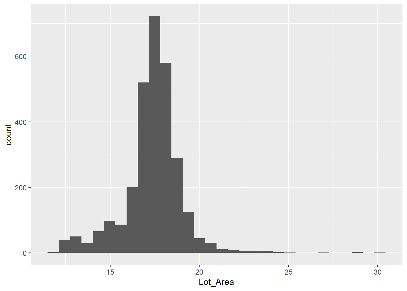

30.1.4 百分位数变换

TODO: https://feaz-book.com/numeric-percentile

30.2 特征缩放

30.2.1 标准化

标准化是将变量转换为均值为0，标准差为1的分布。标准化可以使变量具有相同的尺度，从而提高某些机器学习算法的性能。
标准化不改变变量的分布形状，只会对变量进行尺度的缩放，因此对于高度偏态数据，标准化可能无法改善模型性能。此外，标准化对异常值敏感，异常值可能会显著影响均值和标准差的计算，从而影响标准化的结果。
标准化实际上是先进行center（减去均值），然后进行scale（除以标准差）。

normalize_rec <- recipe(Sale_Price ~ ., data = ames) |>
  step_normalize(all_numeric_predictors()) |>
  prep()
baked_data <- normalize_rec |>
  bake(new_data = NULL) |>
  select(where(is.numeric))
baked_data

# A tibble: 2,930 × 34
   Lot_Frontage Lot_Area Year_Built Year_Remod_Add Mas_Vnr_Area BsmtFin_SF_1
          <dbl>    <dbl>      <dbl>          <dbl>        <dbl>        <dbl>
 1       2.49     2.74       -0.375         -1.16        0.0610       -0.975
 2       0.667    0.187      -0.342         -1.12       -0.566         0.816
 3       0.697    0.523      -0.442         -1.26        0.0386       -1.42 
 4       1.06     0.128      -0.111         -0.780      -0.566        -1.42 
 5       0.488    0.467       0.848          0.658      -0.566        -0.527
 6       0.608   -0.0216      0.881          0.658      -0.454        -0.527
 7      -0.497   -0.663       0.980          0.802      -0.566        -0.527
 8      -0.437   -0.653       0.683          0.371      -0.566        -1.42 
 9      -0.557   -0.604       0.782          0.562      -0.566        -0.527
10       0.0702  -0.336       0.914          0.706      -0.566         1.26 
# ℹ 2,920 more rows
# ℹ 28 more variables: BsmtFin_SF_2 <dbl>, Bsmt_Unf_SF <dbl>,
#   Total_Bsmt_SF <dbl>, First_Flr_SF <dbl>, Second_Flr_SF <dbl>,
#   Gr_Liv_Area <dbl>, Bsmt_Full_Bath <dbl>, Bsmt_Half_Bath <dbl>,
#   Full_Bath <dbl>, Half_Bath <dbl>, Bedroom_AbvGr <dbl>, Kitchen_AbvGr <dbl>,
#   TotRms_AbvGrd <dbl>, Fireplaces <dbl>, Garage_Cars <dbl>,
#   Garage_Area <dbl>, Wood_Deck_SF <dbl>, Open_Porch_SF <dbl>, …

30.2.2 最大最小值缩放

最大最小值缩放的核心目的是将变量压缩至预定义的区间范围内，通常为[0, 1]，以消除因量纲不同或数值范围差异带来的影响。

range_rec <- recipe(Sale_Price ~ ., data = ames) |>
  step_range(all_numeric_predictors()) |>
  prep()
baked_data <- range_rec |>
  bake(new_data = NULL) |>
  select(where(is.numeric))
baked_data

# A tibble: 2,930 × 34
   Lot_Frontage Lot_Area Year_Built Year_Remod_Add Mas_Vnr_Area BsmtFin_SF_1
          <dbl>    <dbl>      <dbl>          <dbl>        <dbl>        <dbl>
 1        0.450   0.142       0.638          0.167       0.07          0.286
 2        0.256   0.0482      0.645          0.183       0             0.857
 3        0.259   0.0606      0.623          0.133       0.0675        0.143
 4        0.297   0.0461      0.696          0.3         0             0.143
 5        0.236   0.0586      0.906          0.8         0             0.429
 6        0.249   0.0406      0.913          0.8         0.0125        0.429
 7        0.131   0.0169      0.935          0.85        0             0.429
 8        0.137   0.0173      0.870          0.7         0             0.143
 9        0.125   0.0191      0.891          0.767       0             0.429
10        0.192   0.0290      0.920          0.817       0             1    
# ℹ 2,920 more rows
# ℹ 28 more variables: BsmtFin_SF_2 <dbl>, Bsmt_Unf_SF <dbl>,
#   Total_Bsmt_SF <dbl>, First_Flr_SF <dbl>, Second_Flr_SF <dbl>,
#   Gr_Liv_Area <dbl>, Bsmt_Full_Bath <dbl>, Bsmt_Half_Bath <dbl>,
#   Full_Bath <dbl>, Half_Bath <dbl>, Bedroom_AbvGr <dbl>, Kitchen_AbvGr <dbl>,
#   TotRms_AbvGrd <dbl>, Fireplaces <dbl>, Garage_Cars <dbl>,
#   Garage_Area <dbl>, Wood_Deck_SF <dbl>, Open_Porch_SF <dbl>, …

30.2.3 Robust

与标准化类似，稳健缩放是通过先减去中位数，然后除以四分位距²来实现的。
与标准化不同，文件缩放不依赖与均值和方差，不受异常值的影响，但在方差接近0的数据无法使用(\(Q1(x) - Q3(x) = 0\))。
稳健缩放的方法不在tidymodels默认加载的包中，需要调用extrasteps包。

robust_rec <- recipe(Sale_Price ~ ., data = ames) |>
  extrasteps::step_robust(all_numeric_predictors()) |>
  prep()
baked_data <- robust_rec |>
  bake(new_data = NULL) |>
  select(where(is.numeric))
baked_data

# A tibble: 2,930 × 34
   Lot_Frontage Lot_Area Year_Built Year_Remod_Add Mas_Vnr_Area BsmtFin_SF_1
          <dbl>    <dbl>      <dbl>          <dbl>        <dbl>        <dbl>
 1       2.23      5.43      -0.277        -0.846         0.688        -0.25
 2       0.486     0.531     -0.255        -0.821         0             0.75
 3       0.514     1.17      -0.319        -0.897         0.664        -0.5 
 4       0.857     0.419     -0.106        -0.641         0            -0.5 
 5       0.314     1.07       0.511         0.128         0             0   
 6       0.429     0.132      0.532         0.128         0.123         0   
 7      -0.629    -1.10       0.596         0.205         0             0   
 8      -0.571    -1.08       0.404        -0.0256        0            -0.5 
 9      -0.686    -0.984      0.468         0.0769        0             0   
10      -0.0857   -0.471      0.553         0.154         0             1   
# ℹ 2,920 more rows
# ℹ 28 more variables: BsmtFin_SF_2 <dbl>, Bsmt_Unf_SF <dbl>,
#   Total_Bsmt_SF <dbl>, First_Flr_SF <dbl>, Second_Flr_SF <dbl>,
#   Gr_Liv_Area <dbl>, Bsmt_Full_Bath <dbl>, Bsmt_Half_Bath <dbl>,
#   Full_Bath <dbl>, Half_Bath <dbl>, Bedroom_AbvGr <dbl>, Kitchen_AbvGr <dbl>,
#   TotRms_AbvGrd <dbl>, Fireplaces <dbl>, Garage_Cars <dbl>,
#   Garage_Area <dbl>, Wood_Deck_SF <dbl>, Open_Porch_SF <dbl>, …

30.3 非线性关系

30.3.1 分箱-binning

分箱本质是将连续的 “数值变量曲线”（比如年龄、收入这类连续数据的分布趋势）拆分成多个离散的 “区间段”（即 “箱”），把原本连续的数值关系转化为更易处理的区间关系。
分箱可以解决 “非线性关系建模难” 的问题：很多模型（如线性回归）天生只能处理预测变量（如年龄）和结果（如消费金额）之间的线性关系，而分箱能将两者间的非线性趋势（比如 “20-30 岁消费增长快，30-45 岁增长平缓”）拆解成多个区间的线性关系，让模型可识别。

binning_rec <- recipe(Sale_Price ~ ., data = ames) |>
  step_discretize(Lot_Area) |> # 创建一个因子变量
  step_dummy(Lot_Area) |> # 将因子变量转换为哑变量
  prep()
baked_data <- binning_rec |>
  bake(new_data = NULL)
baked_data |>
  select(starts_with("Lot_Area")) |>
  glimpse()

Rows: 2,930
Columns: 3
$ Lot_Area_bin2 <dbl> 0, 0, 0, 0, 0, 0, 0, 0, 0, 1, 0, 1, 1, 0, 0, 0, 0, 0, 0,…
$ Lot_Area_bin3 <dbl> 0, 0, 0, 1, 0, 1, 0, 0, 0, 0, 1, 0, 0, 1, 0, 0, 0, 1, 0,…
$ Lot_Area_bin4 <dbl> 1, 1, 1, 0, 1, 0, 0, 0, 0, 0, 0, 0, 0, 0, 0, 1, 1, 0, 1,…

30.3.2 样条函数-splines

可将与目标变量存在非线性关系的数值型预测变量，转化为 1 个或多个与-目标变量呈线性关系的变量。
转换后会产生相关特征（相邻特征高度相关，间隔较远特征呈负相关），需结合 “相关数据处理” 模块方法优化（如高相关性过滤）。
使用样条函数有以下几点需要注意：
- 自由度（deg_free）需谨慎选择：过小可能欠拟合，过大可能过拟合（可通过交叉验证优化）。
- 样条会增加特征维度（如自由度为 5 会生成 5 个基函数），但 tidymodels 会自动处理。
- 自然样条（step_ns()）比 B 样条更稳健，尤其在数据范围外的外推场景。

spline_rec <- recipe(~Lot_Area, data = ames) |>
  # step_bs(Lot_Area) |>
  step_ns(Lot_Area, deg_free = 6, keep_original_cols = T) |>
  prep()
spline_rec

spline_rec |>
  bake(new_data = NULL) |>
  glimpse()

Rows: 2,930
Columns: 7
$ Lot_Area      <int> 31770, 11622, 14267, 11160, 13830, 9978, 4920, 5005, 538…
$ Lot_Area_ns_1 <dbl> 0.000000e+00, 0.000000e+00, 0.000000e+00, 0.000000e+00, …
$ Lot_Area_ns_2 <dbl> 0.0000000000, 0.0474691990, 0.0000000000, 0.1309374466, …
$ Lot_Area_ns_3 <dbl> 0.7245485215, 0.9418727536, 0.9523187732, 0.8632741726, …
$ Lot_Area_ns_4 <dbl> 0.2159072922, 0.0088951108, 0.0395697635, 0.0048329027, …
$ Lot_Area_ns_5 <dbl> 9.139338e-02, 3.534438e-03, 1.581289e-02, 1.919545e-03, …
$ Lot_Area_ns_6 <dbl> -3.184920e-02, -1.771501e-03, -7.701424e-03, -9.640667e-…

# visualize the basis functions
spline_rec |>
  bake(new_data = NULL) |>
  pivot_longer(
    c(starts_with("Lot_Area_ns_")),
    names_to = "feature",
    values_to = "value"
  ) |>
  mutate(feature = gsub("Lot_Area_ns_", "feature ", feature)) |>
  ggplot(aes(Lot_Area, value, color = feature)) +
  geom_line() +
  facet_wrap(~feature)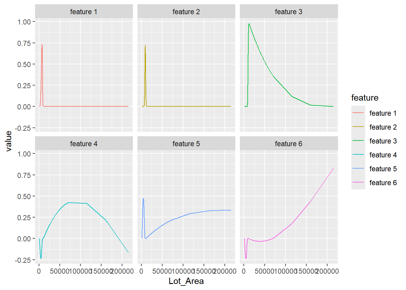

30.3.3 多项式-polynomials

许多模型无法直接处理非线性关系，多项式展开可将与目标变量呈非线性关系的数值变量，转化为一个或多个与目标变量呈线性关系的变量，助力模型有效建模。

与分箱和样条一样，多项式展开也是一种非线性关系转化为线性关系。它的优点是不会像样条那样增加太多特征维度（假设原始变量为 \(x\)，多项式展开后只会生成 \(x^2, x^3, \ldots, x^d\) 这 \(d-1\) 个新变量），但缺点是无法像样条那样灵活拟合复杂的非线性关系，其可解释性也不及样条。

poly_rec <- recipe(~Lot_Area, data = ames) |>
  step_poly(Lot_Area, degree = 3, keep_original_cols = TRUE) |>
  prep()
poly_rec |>
  bake(new_data = NULL) |>
  glimpse()

Rows: 2,930
Columns: 4
$ Lot_Area        <int> 31770, 11622, 14267, 11160, 13830, 9978, 4920, 5005, 5…
$ Lot_Area_poly_1 <dbl> 5.070030e-02, 3.456477e-03, 9.658577e-03, 2.373161e-03…
$ Lot_Area_poly_2 <dbl> -0.052288355, -0.006139895, -0.013560043, -0.004801598…
$ Lot_Area_poly_3 <dbl> 0.0024951091, 0.0067956902, 0.0110336270, 0.0058890125…

大多数数据点分布于较低值的分布。↩︎
第三四分位数与第一四分位数。↩︎