附录 F — gt包-整洁的建立表格

R表格包太多太乱了让人不知道用哪个。gt包是Posit出品，秉承ggplot2理念，再加上它的扩展包gtsummary包（学术），gto包（导出到word，PPT），tablespan包（导出到Excel），会出现一统的趋势。

我们可以将展示表格视为仅用于输出，不希望再次将其用作输入。其他功能包括注释、表格元素样式和文本转换，这些都有助于更清晰地传达主题内容。

注意，我们要展示的表格最好不再参与之后的处理，而是要展示的最终结果。

F.1 gt包的简单表格入门

library(tidyverse)
library(gt)

我们用islands数据集来演示gt包的基本用法。islands数据集实际为一个数字型的向量，包含世界各地岛屿的面积（平方英里）。我们将其转换为数据框以便使用gt包。

# Take the `islands` dataset and use some
# dplyr functionality to obtain the ten
# biggest islands in the world
islands_tbl <- tibble(
  name = names(islands),
  size = islands
) |> 
  slice_max(size, n = 10)
islands_tbl

# A tibble: 10 × 2
   name           size
   <chr>         <dbl>
 1 Asia          16988
 2 Africa        11506
 3 North America  9390
 4 South America  6795
 5 Antarctica     5500
 6 Europe         3745
 7 Australia      2968
 8 Greenland       840
 9 New Guinea      306
10 Borneo          280

接下来，我们使用gt()函数将数据框转换为gt表格对象。

# Create a gt table
gt_tbl <- gt(islands_tbl)
gt_tbl # print the gt table as html widget

name	size
Asia	16988
Africa	11506
North America	9390
South America	6795
Antarctica	5500
Europe	3745
Australia	2968
Greenland	840
New Guinea	306
Borneo	280

在以上表格的基础上，根据 图 F.1 为gt_tbl对象添加对应的部分。

图 F.1: gt包的表格组成逻辑

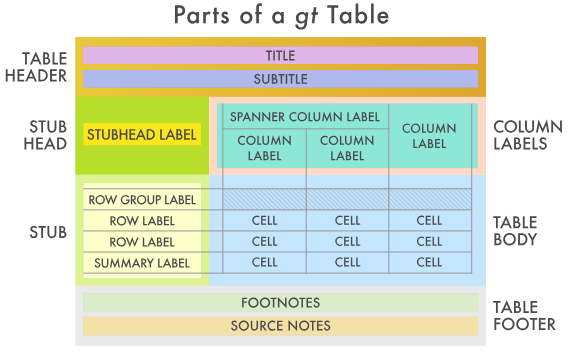
大致包括一下几个部分。

F.2 表头(Table Header)

可选；包含标题和可能的副标题。gt::tab_header()。我们可以使用md()函数在表头的部分使用markdown格式。

# 直接添加标题
gt_tbl_header <- gt_tbl |>
  tab_header(
    title = "Large Landmasses of the World",
    subtitle = "The top ten largest are presented"
  )
gt_tbl_header

Large Landmasses of the World
The top ten largest are presented
name	size
Asia	16988
Africa	11506
North America	9390
South America	6795
Antarctica	5500
Europe	3745
Australia	2968
Greenland	840
New Guinea	306
Borneo	280

# 使用markdown格式
gt_tbl_header <- gt_tbl |>
  tab_header(
    title = md("**Large Landmasses of the World**"), # 加粗
    subtitle = md("The *top ten* largest are presented") # 斜体
  )
gt_tbl_header

Large Landmasses of the World
The top ten largest are presented
name	size
Asia	16988
Africa	11506
North America	9390
South America	6795
Antarctica	5500
Europe	3745
Australia	2968
Greenland	840
New Guinea	306
Borneo	280

F.3 表脚注(Table Footer)

可选；可能包含脚注(gt::tab_footnote())和来源说明(gt::tab_source_note())。相关函数的使用方式与标题函数相同，区别在于它可以被多次调用——每次调用都会添加一个来源说明，每次添加均需要单独使用脚注系列函数。 - cells_*()系列辅助函数，借助columns和rows参数可定位表格的任意单元格。这两个参数可以接受一下几类的输入：（1）列名或行名的向量，（2）列/行索引的向量，（3）用c()包裹的裸列名或用vars()包裹的行标签，或（4）选择辅助函数（starts_with()、ends_with()、contains()、matches()、one_of()和everything()）。特别对于columns，我们可以使用列名作为变量的条件语句（例如colname == value）。

# multiple source note
gt_tbl_sourcenote <- gt_tbl_header |>
  tab_source_note(
    source_note = "Source: The World Almanac and Book of Facts, 1975, page 406."
  ) |>
  tab_source_note(
    source_note = md(
      "Reference: McNeil, D. R. (1977) *Interactive Data Analysis*. Wiley."
    )
  )
gt_tbl_sourcenote

Large Landmasses of the World
The top ten largest are presented
name	size
Asia	16988
Africa	11506
North America	9390
South America	6795
Antarctica	5500
Europe	3745
Australia	2968
Greenland	840
New Guinea	306
Borneo	280
Source: The World Almanac and Book of Facts, 1975, page 406.
Reference: McNeil, D. R. (1977) Interactive Data Analysis. Wiley.

# footnotes with marks attached to cell data
gt_tbl_footnote <- gt_tbl_sourcenote |>
  tab_footnote(
    footnote = "The Americas",
    locations = cells_body(columns = name, rows = 3:4)
  )
gt_tbl_footnote

Large Landmasses of the World
The top ten largest are presented
name	size
Asia	16988
Africa	11506
North America1	9390
South America1	6795
Antarctica	5500
Europe	3745
Australia	2968
Greenland	840
New Guinea	306
Borneo	280
1 The Americas
Source: The World Almanac and Book of Facts, 1975, page 406.
Reference: McNeil, D. R. (1977) Interactive Data Analysis. Wiley.

# Slightly more complex example of adding footnotes
## 寻找拥有最大面积的州
largest <- 
  islands_tbl |> 
  slice_max(size, n = 1) |> 
  pull(name)
largest

[1] "Asia"

## 建立多个footnotes
gt_tbl_footnote_2 <- gt_tbl_footnote |> 
  tab_footnote(
    footnote = md("The **largest** island by area."),
    locations = cells_body(
      columns = size,
      rows = name == largest
    )
  ) |> 
  tab_footnote(
    footnote = "The lowest by area.",
    locations = cells_body(
      columns = size,
      rows = size == min(size)
    )
  )
gt_tbl_footnote_2

Large Landmasses of the World
The top ten largest are presented
name	size
Asia	1 16988
Africa	11506
North America2	9390
South America2	6795
Antarctica	5500
Europe	3745
Australia	2968
Greenland	840
New Guinea	306
Borneo	3 280
1 The largest island by area.
2 The Americas
3 The lowest by area.
Source: The World Almanac and Book of Facts, 1975, page 406.
Reference: McNeil, D. R. (1977) Interactive Data Analysis. Wiley.

F.4 存根与存根标题(the Stub and the Stub Head)

可选；包含行标签，可选择性地置于行组内，行组可带有行组标签，且在存在汇总时可能包含汇总标签。gt::tab_stubhead()。

Stub表侧栏是表格左侧的区域，包含行标签，可能包含行组标签和汇总标签。这些子部分可以按行组顺序进行分组。表侧栏标题为描述表侧栏的标签提供位置。表侧栏是可选的，因为在某些情况下表侧栏并不实用（例如，之前展示的表格在没有表侧栏的情况下也能正常显示）。

可以简单的理解为行名列。

gt_tbl_stab <- islands_tbl |> 
  gt(rowname_col = "name") |> # stub列
  tab_stubhead(label = "landmass") # stub列名
gt_tbl_stab

landmass	size
Asia	16988
Africa	11506
North America	9390
South America	6795
Antarctica	5500
Europe	3745
Australia	2968
Greenland	840
New Guinea	306
Borneo	280

这里需要特别注意的一点是，在没有存根列时，表格有两列（列标签为 name 和 size ），但现在第 1 列（唯一的一列）是 size 。也可以理解为stub列是不算在gt表格的主体中的。

再添加了stub列后，我们就可以使用tab_row_group()函数将行划分为不同的组别，并在每个组的上方显示组标签。

# 添加gt表格各个组件
gt_tbl <-
  gt_tbl_stab |>
  tab_header(
    title = "Large Landmasses of the World",
    subtitle = "The top ten largest are presented"
  ) |>
  tab_source_note(
    source_note = "Source: The World Almanac and Book of Facts, 1975, page 406."
  ) |>
  tab_source_note(
    source_note = md(
      "Reference: McNeil, D. R. (1977) *Interactive Data Analysis*. Wiley."
    )
  ) |>
  tab_footnote(
    footnote = md("The **largest** by area."),
    locations = cells_body(
      columns = size,
      rows = largest
    )
  ) |>
  tab_footnote(
    footnote = "The lowest by population.",
    locations = cells_body(
      columns = size,
      rows = contains("arc")
    )
  )
gt_tbl

Large Landmasses of the World
The top ten largest are presented
landmass	size
Asia	1 16988
Africa	11506
North America	9390
South America	6795
Antarctica	2 5500
Europe	3745
Australia	2968
Greenland	840
New Guinea	306
Borneo	280
1 The largest by area.
2 The lowest by population.
Source: The World Almanac and Book of Facts, 1975, page 406.
Reference: McNeil, D. R. (1977) Interactive Data Analysis. Wiley.

# 行分组
gt_tbl_rowgroup <- gt_tbl |>
  tab_row_group(
    label = md("**continent**"),
    rows = 1:6
  ) |>
  tab_row_group(
    label = "country",
    rows = c("Australia", "Greenland")
  ) |> 
  tab_row_group(
    label = "Subregion",
    rows = c("New Guinea", "Borneo")
  )

gt_tbl_rowgroup

Large Landmasses of the World
The top ten largest are presented
landmass	size
Subregion
New Guinea	306
Borneo	280
country
Australia	2968
Greenland	840
continent
Asia	1 16988
Africa	11506
North America	9390
South America	6795
Antarctica	2 5500
Europe	3745
1 The largest by area.
2 The lowest by population.
Source: The World Almanac and Book of Facts, 1975, page 406.
Reference: McNeil, D. R. (1977) Interactive Data Analysis. Wiley.

提示

创建行分组的另一种方法是在输入数据表中包含一个分组名称的列。以我们上述的 islands_tbl 为例，若在适当行中设置包含 continent 、 country 和 subregion 类别的 groupname 列，当使用 gt() 函数的 groupname_col 参数时（例如 gt(islands_tbl, rowname_col = "name", groupname_col = "groupname") |> ... ），就会生成行分组。这样就不再需要使用 tab_row_group() 。

这种在列中提供分组名称的策略有时更具优势，因为我们可以依赖诸如 dplyr 中的函数来生成类别（例如使用 case_when() 或 if_else() ）。

具体例子可参看gt()函数的帮助说明。

F.5 列标签(Column Labels)

包含列标签，可选择位于跨列标签下方。

表格的列标签部分至少包含列及其列标签。上一个示例中有一个单独的列： size 。正如在存根(Stub)中一样，我们可以创建称为跨列的分组，这些分组包含一个或多个列。tab_spanner()函数的功能正是如此。

我们使用包含更多列的airquality为例。

# Modify the `airquality` dataset by adding the year
# of the measurements (1973) and limiting to 10 rows
airquality_m <-
  airquality |>
  mutate(Year = 1973L) |>
  slice(1:10)
airquality_m

   Ozone Solar.R Wind Temp Month Day Year
1     41     190  7.4   67     5   1 1973
2     36     118  8.0   72     5   2 1973
3     12     149 12.6   74     5   3 1973
4     18     313 11.5   62     5   4 1973
5     NA      NA 14.3   56     5   5 1973
6     28      NA 14.9   66     5   6 1973
7     23     299  8.6   65     5   7 1973
8     19      99 13.8   59     5   8 1973
9      8      19 20.1   61     5   9 1973
10    NA     194  8.6   69     5  10 1973

# Create a display table using the `airquality_m`
# dataset; arrange columns into groups
gt_tbl_air <- airquality_m |>
  gt() |>
  tab_header(
    title = "New York Air Quality Measurements",
    subtitle = "Daily measurements in New York City (May 1-10, 1973)"
  ) |>
  tab_spanner(
    label = "Time",
    columns = c(Year, Month, Day)
  ) |>
  tab_spanner(
    label = "Measurement",
    columns = c(Ozone, Solar.R, Wind, Temp)
  )

gt_tbl_air

New York Air Quality Measurements
Daily measurements in New York City (May 1-10, 1973)
Measurement				Time
Ozone	Solar.R	Wind	Temp	Year	Month	Day
41	190	7.4	67	1973	5	1
36	118	8.0	72	1973	5	2
12	149	12.6	74	1973	5	3
18	313	11.5	62	1973	5	4
NA	NA	14.3	56	1973	5	5
28	NA	14.9	66	1973	5	6
23	299	8.6	65	1973	5	7
19	99	13.8	59	1973	5	8
8	19	20.1	61	1973	5	9
NA	194	8.6	69	1973	5	10

以上gt_tbl_ari表格已经比较美观，但我们还可以进一步美化：

• 将 Time 列移至序列的开头: 使用 cols_move_to_start()。
• 自定义列标签，使其更具描述性: 使用 cols_label()。

gt_tbl_air_modify <- gt_tbl_air |> 
  cols_move_to_start(
    columns = c(Year, Month, Day)
  ) |> 
  cols_label(
    Ozone = html("Ozone, <br>ppbV"),
    Solar.R = html("Solar.R, <br>cal/m<sup>2</sup>"),
    Wind = html("Wind, <br>mph"),
    Temp = html("Temp, <br>&degF")
  )
gt_tbl_air_modify

New York Air Quality Measurements
Daily measurements in New York City (May 1-10, 1973)
Time			Measurement
Year	Month	Day	Ozone, ppbV	Solar.R, cal/m2	Wind, mph	Temp, &degF
1973	5	1	41	190	7.4	67
1973	5	2	36	118	8.0	72
1973	5	3	12	149	12.6	74
1973	5	4	18	313	11.5	62
1973	5	5	NA	NA	14.3	56
1973	5	6	28	NA	14.9	66
1973	5	7	23	299	8.6	65
1973	5	8	19	99	13.8	59
1973	5	9	8	19	20.1	61
1973	5	10	NA	194	8.6	69