30 用yardstick衡量模型性能

library(tidyverse)
library(tidymodels)
tidymodels::tidymodels_prefer()

data(ames)
ames <- ames |>
  mutate(Sale_Price = log10(Sale_Price))

set.seed(502)
ames_split <- initial_split(ames, prop = 0.80, strata = Sale_Price)
ames_train <- training(ames_split)
ames_test <- testing(ames_split)

ames_rec <- recipe(
  Sale_Price ~ Neighborhood +
    Gr_Liv_Area +
    Year_Built +
    Bldg_Type +
    Latitude +
    Longitude,
  data = ames_train
) |> 
  step_log(Gr_Liv_Area, base = 10) |> 
  step_other(Neighborhood, threshold = 0.01) |> 
  step_dummy(all_nominal_predictors()) |> 
  step_interact(~ Gr_Liv_Area:starts_with("Bldg_Type")) |> 
  step_ns(Latitude, Longitude,deg_free = 20)

lm_model <- linear_reg() |>
  set_engine("lm")

lm_wflow <- workflow() |>
  add_model(lm_model) |>
  add_recipe(ames_rec)

lm_fit <- fit(lm_wflow, ames_train)

yardstick包是tidymodels的核心包之一，用于衡量模型的性能。

30.1 回归模型

ames_test_res <- predict(lm_fit, new_data = ames_test |> select(-Sale_Price))
ames_test_res <- bind_cols(
  ames_test_res, ames_test |> select(Sale_Price)
)
ames_test_res

# A tibble: 588 × 2
   .pred Sale_Price
   <dbl>      <dbl>
 1  5.07       5.02
 2  5.31       5.39
 3  5.28       5.28
 4  5.33       5.28
 5  5.30       5.28
 6  5.24       5.26
 7  5.67       5.73
 8  5.52       5.60
 9  5.34       5.32
10  5.00       4.98
# ℹ 578 more rows

# rmse:均方根误差，MAE:绝对平均误差，R2:真实值与预测值之间的平方相关性
rmse(ames_test_res, truth = Sale_Price, estimate = .pred)

# A tibble: 1 × 3
  .metric .estimator .estimate
  <chr>   <chr>          <dbl>
1 rmse    standard      0.0736

ames_metrics <- metric_set(rmse, rsq, mae)
ames_metrics(ames_test_res, truth = Sale_Price, estimate = .pred)

# A tibble: 3 × 3
  .metric .estimator .estimate
  <chr>   <chr>          <dbl>
1 rmse    standard      0.0736
2 rsq     standard      0.836 
3 mae     standard      0.0549

30.2 二分类数据

modeldata包中的two_class_example数据集：

结果变量truth为二分类变量：class1和class2；
数据还包括了模型的预测类别及其预测概率。

data(two_class_example)
tibble(two_class_example)

# A tibble: 500 × 4
   truth   Class1   Class2 predicted
   <fct>    <dbl>    <dbl> <fct>    
 1 Class2 0.00359 0.996    Class2   
 2 Class1 0.679   0.321    Class1   
 3 Class2 0.111   0.889    Class2   
 4 Class1 0.735   0.265    Class1   
 5 Class2 0.0162  0.984    Class2   
 6 Class1 0.999   0.000725 Class1   
 7 Class1 0.999   0.000799 Class1   
 8 Class1 0.812   0.188    Class1   
 9 Class2 0.457   0.543    Class2   
10 Class2 0.0976  0.902    Class2   
# ℹ 490 more rows

# 混淆矩阵
conf_mat(two_class_example, truth = truth, estimate = predicted)

          Truth
Prediction Class1 Class2
    Class1    227     50
    Class2     31    192

# 准确率
accuracy(two_class_example, truth = truth, estimate = predicted)

# A tibble: 1 × 3
  .metric  .estimator .estimate
  <chr>    <chr>          <dbl>
1 accuracy binary         0.838

# 马修斯相关系数和F1值
mcc(two_class_example, truth = truth, estimate = predicted) # 同时关注正负两类的预测质量

# A tibble: 1 × 3
  .metric .estimator .estimate
  <chr>   <chr>          <dbl>
1 mcc     binary         0.677

f_meas(two_class_example, truth = truth, estimate = predicted) # 关注正类的预测质量

# A tibble: 1 × 3
  .metric .estimator .estimate
  <chr>   <chr>          <dbl>
1 f_meas  binary         0.849

# event_level参数指定结果是基于正类还是负类，默认值是结果变量(因子型)的第一个水平
f_meas(two_class_example, truth = truth, estimate = predicted, event_level = "second")

# A tibble: 1 × 3
  .metric .estimator .estimate
  <chr>   <chr>          <dbl>
1 f_meas  binary         0.826

# 多个指标
classification_metrics <- metric_set(accuracy, mcc, f_meas)
classification_metrics(two_class_example, truth = truth, estimate = predicted)

# A tibble: 3 × 3
  .metric  .estimator .estimate
  <chr>    <chr>          <dbl>
1 accuracy binary         0.838
2 mcc      binary         0.677
3 f_meas   binary         0.849

two_class_curve <- roc_curve(two_class_example, truth, Class1) # 计算构成ROC曲线的数据点
two_class_curve

# A tibble: 502 × 3
   .threshold specificity sensitivity
        <dbl>       <dbl>       <dbl>
 1 -Inf           0                 1
 2    1.79e-7     0                 1
 3    4.50e-6     0.00413           1
 4    5.81e-6     0.00826           1
 5    5.92e-6     0.0124            1
 6    1.22e-5     0.0165            1
 7    1.40e-5     0.0207            1
 8    1.43e-5     0.0248            1
 9    2.38e-5     0.0289            1
10    3.30e-5     0.0331            1
# ℹ 492 more rows

roc_auc(two_class_example, truth, Class1) # 计算ROC曲线下面积

# A tibble: 1 × 3
  .metric .estimator .estimate
  <chr>   <chr>          <dbl>
1 roc_auc binary         0.939

autoplot(two_class_curve) # 绘制ROC曲线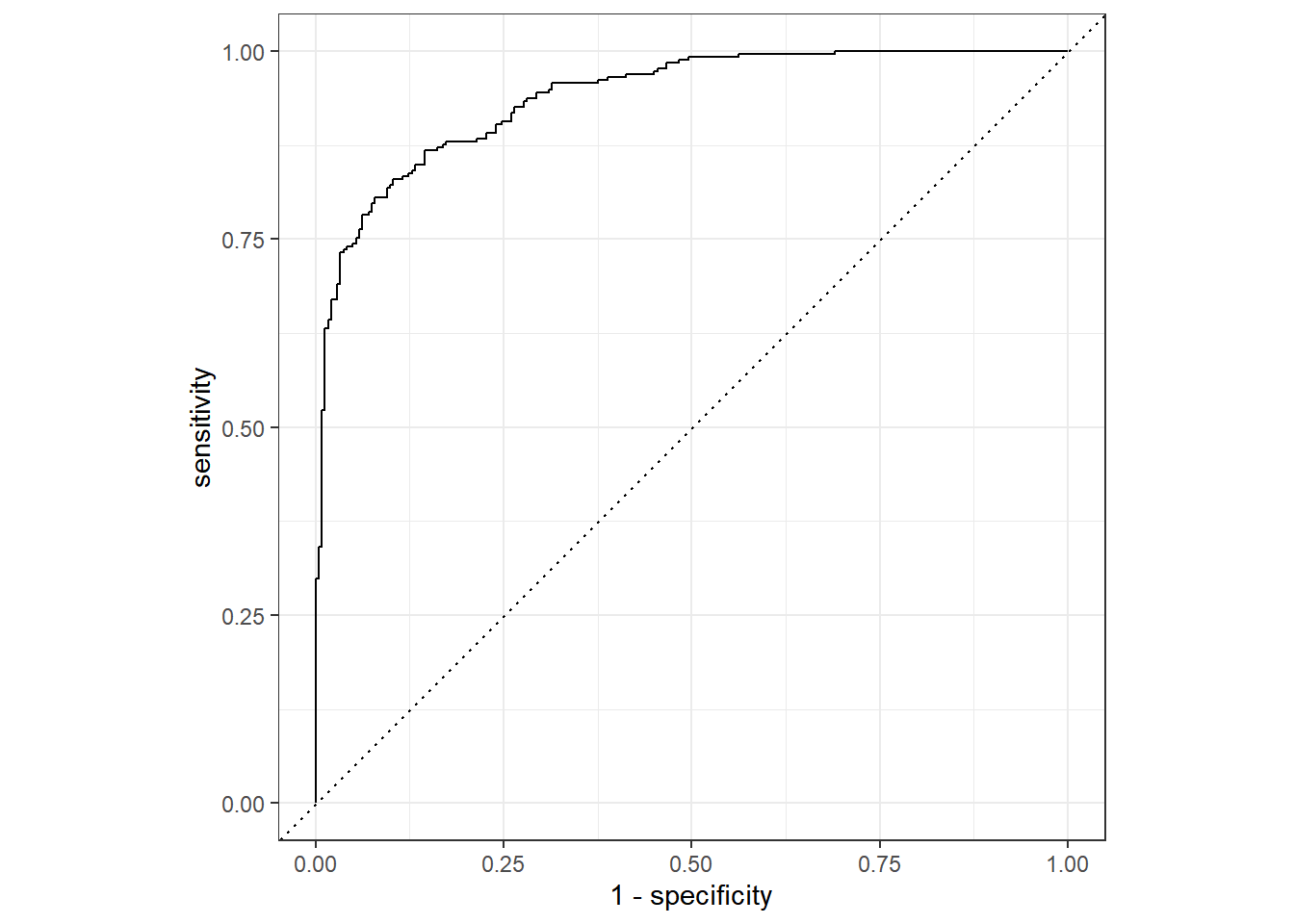

30.3 多分类数据

data(hpc_cv)
tibble(hpc_cv)

# A tibble: 3,467 × 7
   obs   pred     VF      F       M          L Resample
   <fct> <fct> <dbl>  <dbl>   <dbl>      <dbl> <chr>   
 1 VF    VF    0.914 0.0779 0.00848 0.0000199  Fold01  
 2 VF    VF    0.938 0.0571 0.00482 0.0000101  Fold01  
 3 VF    VF    0.947 0.0495 0.00316 0.00000500 Fold01  
 4 VF    VF    0.929 0.0653 0.00579 0.0000156  Fold01  
 5 VF    VF    0.942 0.0543 0.00381 0.00000729 Fold01  
 6 VF    VF    0.951 0.0462 0.00272 0.00000384 Fold01  
 7 VF    VF    0.914 0.0782 0.00767 0.0000354  Fold01  
 8 VF    VF    0.918 0.0744 0.00726 0.0000157  Fold01  
 9 VF    VF    0.843 0.128  0.0296  0.000192   Fold01  
10 VF    VF    0.920 0.0728 0.00703 0.0000147  Fold01  
# ℹ 3,457 more rows

# 衡量指标
accuracy(hpc_cv, truth = obs, estimate = pred)

# A tibble: 1 × 3
  .metric  .estimator .estimate
  <chr>    <chr>          <dbl>
1 accuracy multiclass     0.709

mcc(hpc_cv, obs, pred)

# A tibble: 1 × 3
  .metric .estimator .estimate
  <chr>   <chr>          <dbl>
1 mcc     multiclass     0.515

部分指标是基于二分类数据设计的，在yardstick中，只需在相应函数中指定estimator参数即可。
ROC曲线同样可以应用于多分类数据，但必须将所有预测概率列全部提供给函数才行。也可以指定estimator参数。

roc_auc(hpc_cv, obs, VF, F, M, L)

# A tibble: 1 × 3
  .metric .estimator .estimate
  <chr>   <chr>          <dbl>
1 roc_auc hand_till      0.829